The problem is that of modelling and characterizing heterogeneity in reservoirs in the shallow subsurface of the earth. The classical approach here is to use variograms which are mathematically equivalent to autocovariance functions. However, for an engineer conditional probabilities are easier to interpret than autocovariance functions, which makes modelling by Markov chains attractive. In the simplest model the states of the chain represent the different lithologies like sand, shale and rock. The reservoir is discretised to a certain scale into square regions and the transition matrix of the chain describes the probabilities of transition from one lithology to another. There is a major problem here: Markov chains describe a one-dimensional chain of states, but for reservoirs one would of course prefer a 2d (sections) or 3d description. Since the beginning of the seventies a nice mathematical theory has been developed of objects that generalise Markov chains to higher dimensions - regretfully the objects go under the somewhat confusing name Markov random fields. Even more regretfully engineers do often not like to use Markov random fields. The main reason for this is the problem known as ``the intractability of the normalising constant'', which makes simulations expensive and likelihoods difficult to work with. In Elfeki's model two ordinary Markov chains, one for the horizontal direction and one for the vertical direction, are what he calls ``coupled''3 to generate a two-dimensional image of a section of a reservoir.
The image, built out of rows of
little squares called pixels, is generated from top to bottom and
from left to right by specifying the states in an initial top row
and left column, and then making transitions according to the
following rule: the state of pixel ![]() is deduced from the
states of pixels
is deduced from the
states of pixels ![]() and
and ![]() by
by
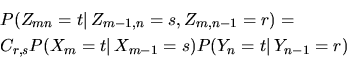
Here ![]() and
and ![]() are the two ordinary Markov chains
representing the horizontal, respectively the vertical direction,
and
are the two ordinary Markov chains
representing the horizontal, respectively the vertical direction,
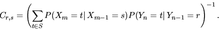
and ![]() is a normalising constant which arises by forcing
transitions in the
is a normalising constant which arises by forcing
transitions in the ![]() and
and ![]() chain to the same
state. Hence, writing
chain to the same
state. Hence, writing ![]() for the set of all states,
for the set of all states,
See Figure 1 for a simulation of a section of a field with 5 different types of lithology. The vertical transition probabilities can be estimated from information from well logs, and the horizontal transition matrix from geological surveys.